St. Paul's Statistics Introduction: Chapter 4 - Gaussian Statistics Problem Solution
Using the Gaussian Probability Distribution to Solve Real World Problems
Section Goals:
- Students will develop an understanding of the Gaussian PDF Equation and Graphic PDF representation.
- Students will develop an understanding of the Standard Normal Distribution as special case of the Gaussian Distribution.
- Students will demonstrate the ability to understand problems and to manipulate PDF 'Z-Tables' to calculate answers to real world problems using Gaussian statistical methods.
Gaussian Probability Function Definition:
The Gaussian Probability Distribution is the familiar 'bell' shaped curve shown in Figure 2 below. In the words of Professor Clifford Swartz, 'In a surprising number of cases, experimental data can be fitted to ... the Gaussian equation.' (see Used Math page 86, Prentice-Hall, Inc., 1973). This reality explains wide spread use of the Gaussian in sociology, education, biology and industry.
The Gaussian PDF is usually shown as a graph where:
- The x axis is used for a random variable (such as IQ scores, bolt strength etc.)
- The y axis is used to indicate frequency of occurrence of corresponding x values.
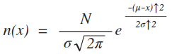
For the Gaussian Distribution, the random variable (x axis) is continuous, thus the PDF graph appears as a smooth curve. The graph form of the PDF is simply a plot of the Gaussian equation shown below.
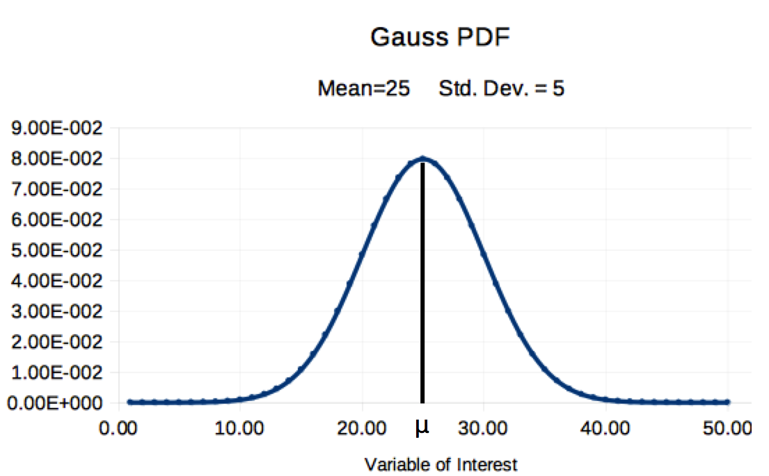
Gaussian PDF Equation
Ch4 Figure 1
Where:
- N = Total number of items. (for percent predictions, N=1 or 100%)
- μ = The mean (or average) value of the population (μ='mew')
- σ = Standard Deviation (the measure of the spread, or width of the PDF) (σ='sigma')
- π = 3.14159
- e = 2.71828
- x = the value along the x axis that traps a range of values who's probability we wish to know.
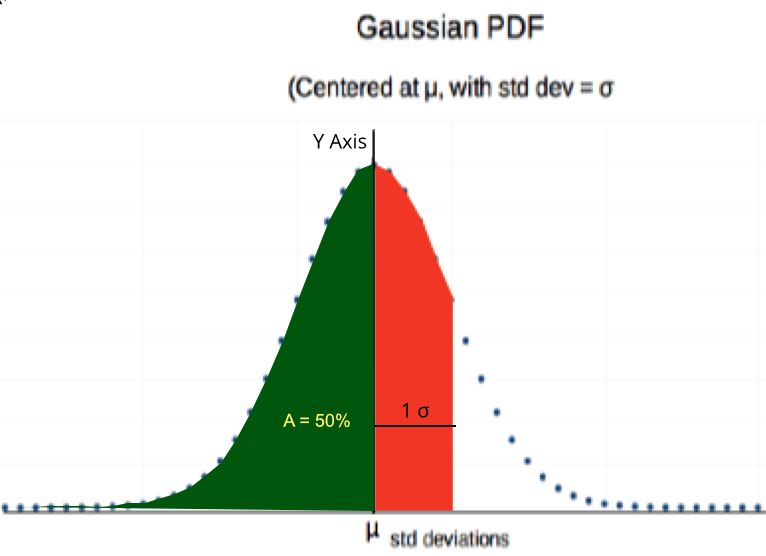
Gauss PDF graph with Area set to 100%
Ch4 Figure 2
Characteristics of the Gaussian Distribution:
Study Ch 4 Figure 2 above and compare its features to the Gaussian PDF characteristics listed below:
- The PDF distribution is right-left symmetric, centered about the mean (μ)
- 50% οf the area is to the left of the mean and 50% is to the right of the mean
- if N of Figure 1 is set to 1 (as illustrated), the area under the curve will be 100% (if N=37, the area will be 37)
- The curve grows wider as the value of the standard deviation (σ) increases. (in concert, the height will shrink, thus keeping area at 100%). Ch 2 Figure 2 provided six examples of how the Gaussian shifts with changes in μ and σ.
- When x is more than three times the std. dev. (σ) from the mean (μ), the PDF curve will drop almost to the y axis. Thus, while the Gaussian is infinitely wide, we can usually ignor the far left and right 'tails'.
Gaussian Distribution Use Criteria:
The Binomial Distribution of Chapter 3 has very clear criteria for use. When the criteria are met, the Binomial Distribution can be used. Unfortunately, the Gaussian has no such clear criteria. The Gaussian Distribution is often selected in the same way an auto mechanic selects a wrench, 'It fits, so I use it'.
How do we know if the Guassian Distribution fits the data? The most frequently used method is to plot the data and see if it looks Gaussian. When many data points are available, the data is put into 'bands or ranges' of values and the midpoint of each band is paired to its count in a spreadsheet. A graph is produced and if it has a 'bell' shaped appearance, the use of the Gaussian is justified. A notional example of banded data and graph for 154 tested bolts is shown below:
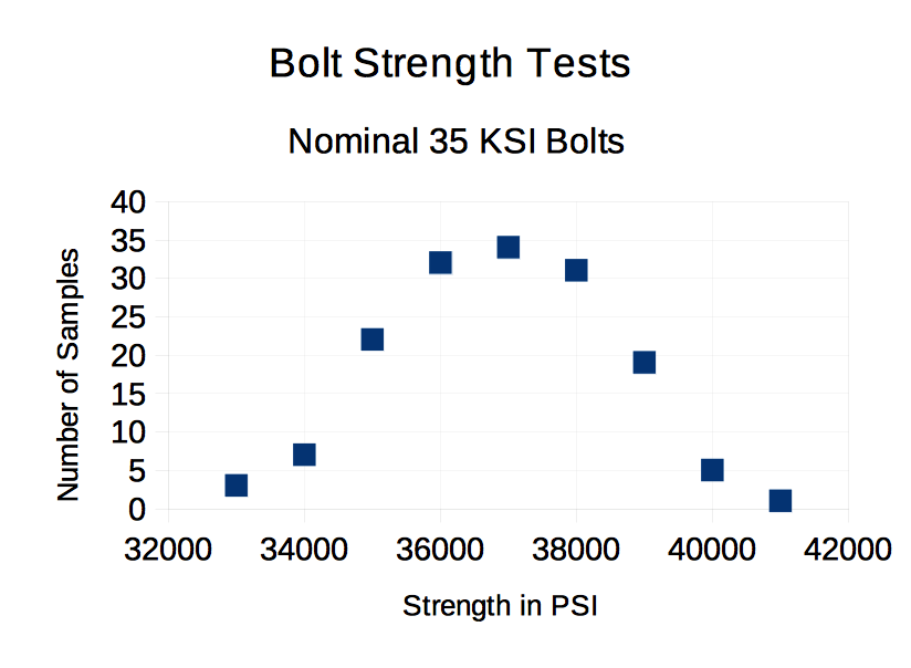
Test Data 'Looks' Gaussian
Ch 4 Figure 3
For the sample of 154 bolts, the data looks Gaussian and this is typical of production from an assembly line. Depending on the application, this visual confirmation may be sufficient justification for using the Gaussian Distribution. There are mathematical ways of justifying use; but, the 'eyeball test' may be the best. From Professor Swartz, 'It is a rare problem in correlation, when better judgement can be drawn from knowledge of r^2 (coefficient of correlation) than can be obtained by examining a scatter diagram of the data (see Used Math). ' In conclusion, a visual confirmation of data to the expected 'bell' shaped curve is usually sufficient basis for using the Gaussian Distribution.
The Mean and the Standard Deviation:
Solving problems using the Gaussian Distribution usually requires knowing two parameters:
- The Mean (or average) symbolized as μ
- The Standard Deviation symbolized as σ
There are two different sources for this data:
- Method 1: The population mean and population standard deviation may be well established from either copious amounts of data, or from well developed theories (such as in Physics). When well established values for μ and σ are available, the analyst proceeds to a direct solution of the problem at hand with confidence that his answer is justified.
- Method 2: A sample of data is used to compute a sample mean (xbar) and a sample standard deviation s (xbar and s are used in lieu of μ and σ for sample data). Unfortunately, if 10 samples of data were analyzed for mean and standard deviation, ten different number pairs would result and there is no method for knowing which of the answers is truly correct. Nevertheless, the analyst proceeds with solution of the problem, but additional steps are needed to provide confidence that the answer is accurate. Chapter 5 will explain how to compute sample values of mean and standard deviation from data. Chapter 5 will also provide a method of justifying confidence in the answer.
Gaussian PDF and Area Representation of Probability
In Chapter 3, specific problem solution using the Binomial Distribution was achieved by picking the correct term from the Binomial Equation and solving it. Unfortunately, the Gaussian PDF does not provide such easy methods because:
- The Gaussian Equation does not have specific terms that correspond to specific probability computations. Worse still, the Calculus math that usually computes areas under a curve does not generally work for the Gaussian PDF Equation.
- Probability Areas under the Gaussian PDF graph cannot be accurately estimated 'by eye'.
Thus, the area under the curve can provide answers; but, previously studied methods for finding that area do not work.
A method for solving Gaussian problems has, however, been developed based on the following:
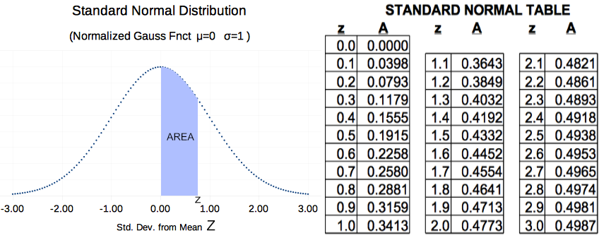
- It is possible to draw a "representative" PDF, with the mean (μ) centered on the y axis and with a standard deviation of one (σ=1). The area under the curve represents 100% (achieved by setting N of Ch 4 Figure 1 to 1). The horozontal axis is labeled 'z'.
- The equation from Figure 1 (with μ=0, σ=1, N=1), is used to analyzed this 'representative' PDF. Computer estimates of the area under the curve are made for many thin slices along 'z' using trapazoidal area (optional) summations. From computer results, a table is built that correlates positions along 'z' with the area trapped. This area 'A' is the probability trapped between the mean and some distance 'z' to the right of the mean.
- Last, a transformation z=(x-μ)/σ is defined. When working a Gaussian statistics problem, the mean (μ), and the standard deviation (σ) will likely be known. Thus the z value can be computed.
- The value of 'z' serves as a bridge between a real world problem and the representative distribution embodied in the Table, Ch 4 Figure 4 below.
Computer Generated 'Z' Table
Ch 4 Figure 4
General Solution Method Summary:
- The analyst rapidly sketches a PDF centered on the mean. Label μ on the z-axis directly beneath the highest point of the graph (mean μ is always the high point)
- Estimate the position of 'z' value (left of μ if desired 'z' is smaller than μ) and mark it on the 'z' axis. You simply guess its position either to the right or left of the mean depending on whether is is greater than or less than μ.
- Compute the z value from the problem where: z = (x-μ)/σ
- Consult Table Figure 4. Reference the Z value, and read corresponding 'A' value. The 'A' value is effectively the percentage of total area (after you slide the decimal 2 places right)
- The PDF sketch is consulted to ensure the 'A' percentage value truely answers the original question. Depending on the problem, the analyst may need to add 50% to account for the area left of the mean. Depending on the problem, the analyst may need to subtract the 'A' percentage from 50%. As stated repeatedly, you must understand the PDF, and then use that basic knowledge along with the percentage value from the Z-Table to get your final answer.
- As a final step, clearly state your answer.
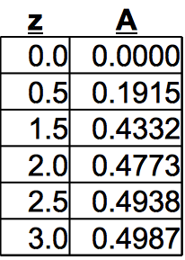
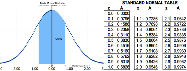
The 'Z-Table':
A method has been summarized for solving problems involving Gaussian distributions. But the table in Ch4 Figure 4 should have more rows, and a small picture to remind the reader of its relationship to the PDF. Figure 5 below addresses these issues.
The picture and 'Z Table' are based on the Standard Normal PDF (Gaussian with μ=0 σ=1 and Area = 100%). The table below descibes the blue area (which is percent) between the mean and some value of z.
A Larger 'Z-Table'
Ch 4 Figure 5
Please recall that for every PDF, area represents percent probability. So for Figure 5, the total area under the curve is 100%. Because Gaussian PDFs are always symmetric, the white area at the left is 50%. The 'blue' shaded area depends on how far 'z' (blue area right edge) extends to the right of center. If z=1, then the blue area would be 34.13% (see table Figure 5). If z=.2, then the blue area would be 7.93% (see 'Z-Table' Figure 5).
Western Oregon Hay Production Example:
For this example, the PDF Figure 5 above represents hay production. Z=0 represents the mean (average) hay production per acre. The white area left of mean, represents the probability that hay yields will be less than average (of course, there is a 50% chance of hay yield being less than average because average is the mid point)
The 'blue area' of Figure 5 represents the probability of production levels between the mean and up to a specific value of Z (the right corner of blue).
Example 1a: The Hay Problem
Average western Oregon hay production is 112 bales per acre with a standard deviation of 26 bales per acre. What is the probability of producing between 112 bales/acre and 125 bales/acre?
- The question amounts to asking how much blue area there is between the mean, and some value of z. It is important that we understand what area in Figure 5 we are talking about. In this problem, we are asked the probability (or area) of exactly the blue area. For this problem, once we 'look up' the blue area, we are done.
- Part a asks us to find the percentage between the mean (middle) and 125 bales/acre. To use the chart in Figure 5, we must first compute z (position of right edge of blue).
- Compute z: z=(x-μ)/σ -> (125-112)/25 -> ~.5 So, z=.5
- Consult Table Figure 5: z=.5 corresponds to 'A'=.1915 or 19.15%
- Answer: About 19% of hay fields in Western Oregon should produce between 112 and 125 bales per acre.
Example 1b: More Hay Questions
The average hay production is still 112 bales/acre with a standard deviation of 26 bales per acre. What is the probability of producing less than 125 bales per acre?
- The numbers in the problem are the same, but the question has changed. We need to figure out the area of PDF Figure 5 that will answer the question.
- Less than 125 bales/acre means we need the blue area (from z=0 to z=.5), but we also need the white area to the left of the mean. That will be EVERYTHING below 125 bales/acre.
- The white area left of mean is 50% from our general knowledge of Gaussian PDFs.
- The blue area is 19.15% (just like it was in part a)
- We need the total of the areas or 50%+19%= 69%
- Answer: The probability of a field producing less than 125 bales/acre is 69%. (and of course, the probability of producing more than 125 is everything else or 31%. This leads us to the next example.)
Example 1c: Hay Problem with Different Question:
The μ and σ are the same as before. What is the probability of producing more than 150 bales per acre?
- Before, we were asked about 125 bales/acre, but now we are asked about 150 bales/acre. Thus we must compute z for the new production value. The question has changed in another way. We are now asked the probability of more than 150 bales/acre. This means we need to figure out the little white area at the far right of the PDF in Figure 5. First, we will figure out everything to the left of 150. Then we will subtract it from 100% leaving us with the answer.
- Compute 'z': z=(x-μ)/σ -> (150-112)/25 -> 1.52
- Now, find the 'A' from Table 5 which represents the blue probability.
- From Table 5, looking up z=1.52 indicates 'A'=.4332 (call it 43%).
- So the area of blue plus the white tail left of mean: 43%+50%=93%
- 93% of hay production is less than 150 bales/acre. So from 93% to 100% is our answer. 7%
- Answer: 7% of hay fields will produce more than 150 bales per acre.
Cow Milk Production:
Internet research indicates that Ayrshire cow herds produce an average of 55 pounds of milk each day with a standard deviation of 7.1 pounds/day (times number of cows). Assume a Gaussian distribution applies and answer the following questions:
Example 2a:What Percent of Cow Herds produce 55 to 62.1 pounds/day?
- Sketch a PDF, showing estimated location of mean and desired data point (62.1#)
Conceptual Sketch - Cow Milk Production
Ch 4 Figure 6
- Estimate position of z value (lower right corner of red region). Use that to shade in the 'red' area shown above.
- Compute z: z=(x-μ)/σ -> (62.5-55)/7.1 -> 1.0
- Consult 'Z Table', Figure 5 above. z=1 corresponds to .3413 or 34.13%. Thus 34.13% of herds will produce between 55 and 62.1 pounds/day (and based on number of cows).
- That is exactly the question asked.
- Answer: 34.13% of herds will produce between 55 and 62.1 pounds/day of milk (times number of cows.)
Example 2b: What percent of cow herds will produce 62.1 lbs/day or less?
- The numbers are the same, but the question has changed. Now, we want the percent for EVERYTHING less than 62.1 pounds which means we must also include the green area to the left of the mean.
- The green area is 50%, because the Gaussian is symmetric. the tail left of mean is always 50%.
- 50% + 34% = 84%
- Answer: 84% of cow herds will produce less than 62.1 pounds per day (for each cow)
When solving a problem in the real world, it is important to understand what μ and σ really mean (i.e. how were they developed?). We need to clearly understand whether μ refers to the the variation between individual cows, or the variation between herds. I must confess that while I was typing up this web page, I had go back to the Internet and verify that those were 'herd' based statistics. This type of cow is present in New Zealand, Scottland and many other countries. I speculate that the conditions vary greatly and so may statistics (μ and σ) from different countries. In conclusion, the analyst should try to ensure that the basis for his statistics (μ and σ) are similar to the problem he is asked to analyze.
Homework Problems:
Work the problems assigned by your instructor. Ε-mail your work or hand it in for evaluation. For Internet Students without instructors, work the even numbered problems. Odd numbered problems may be worked for added practice, or used as examples in class.
1. Biplanes: 'Best Aeroplanes' makes small biplanes for spraying crops with agricultural chemicals. 'Best' buys high strength aluminum to a specification that requires:
- Strength: μ = 50 ksi (i.e. 50000 pounds per square inch) and σ = 2.5 ksi
'Best' performs a test on two samples and measures the strength at 47 ksi and 48 ksi.
a. How likely is it to find a test sample at 47 ksi or less?
b. How likely is it to find a test sample at 48 ksi or less?
c. How likely is it to find two samples in a row like this (see Ch 1 Probability Law 1)
d. Should 'Best' be concerned? What do you suggest they do next?
2. Lilliput Father worries about Daughter's Marriage: In Lilliput, worker wages follow a Gaussian distribution with μ= 21 pesos/week and σ = 3 pesos/week.
a. If Juan earns 21 pesos/week, what percentage of Lilliputions are worse off than Juan?
b. Juan's daughter meets a young man named Ethen and they want to get married. But Juan is worried about Ethen's ability to support a family. Ethen tells the father that he earns 26 pesos per week.
- What percentage of Lilliputions earn less than Ethen?
- Should Juan believe Ethen, or should he be a little cautious with Εthen's answer? Why?
3. Auto Fuel Efficiency Regulations: The 'Environmental Agency' in Lilliput requires all new cars be tested and certified to 30 miles/gallon (or better) fuel efficiency. Assume that production line fuel efficiencies follow a Gaussian distribution.
The newly designed 'X-Car' has a mean fuel eficiency of 40 mpg with a standard deviation of 3 mpg.
a. What percentage of X-Cars will fail their milage test?
b. Out of 1000 cars, about how many cars would you expect to fail?
4. New Car Repairs: Assume auto frequency of repairs follows a Gaussian distribution., Dealer repair records indicate the frequency of new car repairs has a μ = 24 months with σ = 6 months. What percentage of new cars sold will require repairs before one year of use?
5. Automobile Belt Replacement: Lilliput's 'Brand X' automobiles have timing belts with an average life of 110 thousand miles and a standard deviation of 10 thousand miles. What "mainenance milage" should the auto maker recommend to ensure less than .8% (i.e. 008 of cars) breakdown (99.2 don't) on the higway with this expensive type of failure?
6. Education and Reading Speed: Triangle Elementary School carefully monitors it's reading program and evaluates student reading speed (words per minute or wpm). After several years of data collection, Triangle built a graph of student results and found reading speed variation appears to be Gaussian. For the 5th grade, average reading speed was: μ=172 wpm with σ=40 wpm.
a. What is the probability that a student picked at random will read faster than 300 wpm?
b. if the school has 135 5th grade students, then what is a good estimate of the number of students who can read faster than 300 wpm?
c. Can this problem be solved with the binomial distribution? Why?
d. Trick Question: What is the probability that a student picked at random will read exactly 300 wpm? (i.e. between 300 wpm and 300 wpm?)
7. Tire Warantee: Manufacturer 'Nihon Limited' performs testing and learns that Nihon's 'Sterling' tire has a mean life of 35 thousand miles with a standard deviation of 5 thousand miles.
a. What percent of Nihon tires will last 42 thousand or more miles?
b. Nihon has a 100% price refund guarantee if the tire does not last 25 thousand miles. What percent of tires will Nihon end up paying for?
c. If Nihon builds that into the price, what percent extra should Nihon charge for each new tire?
8. Leprosy Sickness Development: the disease Leprosy has a mean development time of 10 years after infection with a standard deviation of 5 years. Assume 100% of exposed people will eventually catch the disease. If all tribe members on the island are exposed from birth, what percentage of the population will have no symptoms at age 12?
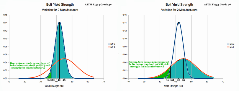
PDF for Two Industrial Processes
Ch 4 Figure 7
9. Which Bolt Manufacturing Method is Best? A factory manager has two alternative manufacturing processes for making 36 ksi (36000 pounds per square inch) foundation bolts. Bolt strength follows a Gaussian distribution. Process 'A; results in a lower average strength, but bolts from this process have little variation in strength (small σ). Process 'B' on average makes a stronger bolts, but the bolts have a lot of variation (large σ).
- Process A: μ = 42 ksi strength
- Process B: μ = 45 ksi strength
The factory manager wants to know which process will produce the fewest number of 'rejects' (i.e. a bolt with strength less than 36 ksi).
See Chapter 4 Figure 7 above, for PDF illustrations of the two processes. You do not need to do math. Just look at the two graphs and figure out the answer. Explain your answer based on the colored areas of the two graphs.
10. Robin Hood: Robin Hood was a famous English archer at the dawn of English history. It is said he could shoot 4 arrows into a 4 inch circle at 200 feet.
Modern Archers Shooting Accuracy: If a modern archer has a target error mean (μ) of 6" at 200 feet and a standard deviation (σ) of 2 inches with a Gaussian distribution, then:
- What is the probability that the modern archer can place one arrow into the 4 inch target at 200 feet?
- What is the probability he can repeat Robin Hoods accomplishment with 4 arrows in a row? (Review Chapter 1 Probability Law 1)
11. Cannon Shell Accuracy: During the Russian-Japanese War in 1904, the Japanese fired high angle cannons at Russian ships anchored in the harbor. Russian ships were 65 feet wide. 30% of the shells hit their targets.
Assume: Fall of shells follows a Gaussian Distribution
Assume: Japanese shell fire was centered on Russian ships
a. What was the standard deviation σ of the Japanese cannon fire?
b. What percentage of Japanese shells would have landed within 5 feet of the ships, but not actually hitting them?
Different Kinds of Z-Tables:
The 'Z Table' and PDF of Chapter 4 Figure 5 match one another. But not all 'Z Tables' look like that. During homework solution, you often ended up adding the area from the 'Z-Table' to 50% (left white tail) to get your final answer. Did you ever wish for a 'Z-Table' that had a picture and table to match the one below? Some 'Z-Tables' are built that way.
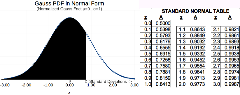
Z-Table That Includes Left Tail
Ch 4 Figure 8
Chapter 4 Figure 5 provides a 'Z-Table' that only shows a blue area to the right of the mean. For Figure 5, if z=1 then A=34% in the Figure 5 table.
Figure 8 above is different. The PDF shaded area once again extends some distance z to right of mean; but, it extends all the way to the far left of the PDF (which goes to infinity by the way). If that is true, the Figure 8 Table should show 50% added onto the 34% for z=1. Looking at Table 8 above, the value shown really is 84%. This is the table that you often wished for during your homework!
Another Kind of 'Z-Table' (Symmetric Shaded Area Around Mean):
There is yet another common kind of 'Z-Table' and it is often used in the Engineering world. This third kind of 'Z-Table' looks like Figure 9 below:
PDF and 'Z-Table': Both + and - z
Ch 4 Figure 9
There are many situations (especially in the Engineering world) where the combined area equi-distant both -z and +z from the mean is desired. Table 9 above may be used in such circumstance (i.e. in lieu of using Figure 5 and doubling the area to account for that equal portion left of μ). Three examples of where this kind of table is preferred follow:
Example 1: The length of a bolt or screw is critical in aircraft engineering applications where control of weight is critical to design success. The monitoring of production requires overall length control. Thus, statistics of analysis must consider length that falls excessivley either to the left or right of the design mid-point. Figure 9 Z-Table above can be used in such situations.
Example 3: Multiple methods exist for analyzing the life of electronic products in a vibration environment. One of the more common methods is to perform a Steinberg analysis (see TBD by David S. Steinberg) which relys on characterizing vibration using a double sided PDF as described by Figure 9 above.
Many Kinds of 'Z-Table': There are many kinds of 'Z-Table' depending on the PDF area that is tabulated against the 'z' value. This is one of several reasons why 'Z-Tables' are generally accompanied by a PDF graph with shaded area. In general, any of them can work for an aware analyst, but students are advised to look critically at the accompanying PDF graph before proceeding with analysis.
Students, Be Ye Aware of 'Z-Table' interpretation!
General Discussion and Conclusions:
- Most statistics books provide 'Z-Tables' with many, many more rows than Ch 4 Figure 5 above. The student should obtain (either from Internet or book) a good 'Z-Table' which includes a small shaded illustration like the one in Ch 4 Figure 5. Get a table that you will be comfortable working with.
- When the 'Z-Table' indicates 47.13%, students should use the full 47.13% (should not round off to 47% as was done in the examples.)
- When z falls between 2 values in the table, the student should use linear interpolation to estimate the value between 'bracketing' z values. Of course, students, like instructors, get lazy and z=2.21 is really rather close to z=2.2
- The analyst generally uses values of μ and σ (else xbar and s for sample values) to solve problems. These should not be used 'blindly'. Whenever possible the analyst should try to verify that μ and σ are based on variation much like the subject of analysis. For example, when we read about μ and σ for milk cow production, we need to understand whether those values were based on herd variation, or based on individual cows. The herd value will have a smaller variation (σ) and this will affect the results of your computations.
- The majority of homework problems presented had μ and σ defined, and a probability was requested. Not all problems are like that. Some problems offer the percentage and mean, and σ must be computed. In the real world, an analyst must often play 'cat and mouse' with the equations until he/she finds a path to solution based on what is known.
Letter to Students:
I hope this brief introduction to solving problems involving the Gaussian Distribution is helpful. Get lots of practice, because Gaussian applications are common in the 'real world'.
When I was doing Internet research in support of homework problems, I had trouble finding information that included both μ and σ. When I did get this information, the basis of its development was often unclear. I was left wondering whether Internet articles are intended for a nontechnical audience, or whether the researchers themselves lacked deep insight into the information they should convey.
I am reminded of a doctor in Cuba who identified the mosquito as carrier of Malaria in the 1870s. He correctly identified the exact type of mosquito; but, he was many years out of college and his scientific presentation was insufficient. Thousands died during Panama Canal construction because of his insufficient technical presentation.
I am hopeful, that this course will give you the technical insight that you need -- the tools that long dead Spanish doctor lacked.
Best Wishes to Your Future,
Paul Watson
Contact the author paul-watson@sbcglobal.net
by e-mail.
© 2019 All Rights Reserved
Paul F. Watson
Beginning
of St. Paul's Statistics Introduction
Dionysus.biz Home Page