St. Pauls Introduction to Statistics

Building a Z-Table by Computerised Trapezoidal Summation (Rev A)

Introduction: From St. Pauls Statistics Introduction we know that the probability of an event falling between z = a and z = b is equal to the area under the PDF curve between those same two values. St. Paul also indicated that Calculus can not determine the area for a region of the Gaussian Distribution (it does work well for many other distributions).

Given our math inability to determine area, we are forced to use computer approximations and document them in a table, commonly called a 'Z-Table'. The 'Z-Table' is married to an idealised Gaussian Distribution centered around the mean (μ=0) with a standard deviation of 1 (σ = 1). Of course, the total area under the curve is 100% (i.e. N=1) because all Probability Density Graphs (PDF) are built that way.

How can we do a computer analysis of area? We can start with the general Gaussian PDF equation and assign μ=0, σ=1 Ν=1. Then we simplify the equation. The result is Figure 1 below. Figure 1 is the equation of the idealised Gaussian Distribution. It is the key to computing Z-Table values:
The Gaussian Defining Equation

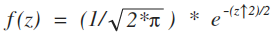
Standard Normal PDF Equation
Figure 1

An explanation of how to find values of area, corresponding to different z values follows. The method is not difficult and can be accomplished by a computer using a spreadsheet.

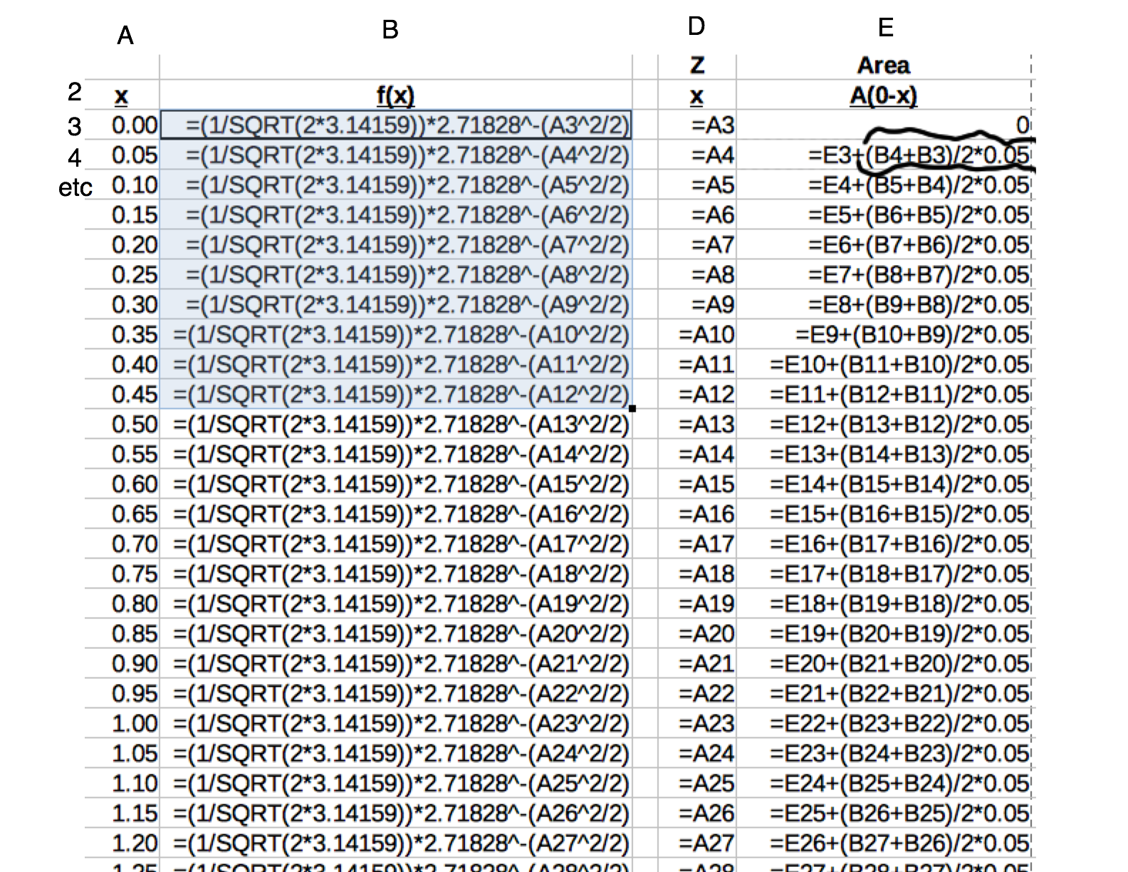
Spreadsheet Implementation of Trapezoidal Area Method
Figure 2

Overview of Trapezoid Area Method: The trapezoidal area approximation is explained in any beginning Calculus book; but, it is simple enough for an algebra student. It works well for computer analysis.

If we want the area under a curve between two points (points a & f, both on the x axis), the area is divided into vertical strips of uniform width w. We then calculate the height of each strip & multiply by w to get the area for that strip. Finally, we add up all the strips for the region of interest. When using this method, I usually define the left an right boundaries of the region as x=a, x=f (a and f are numbers) as shown in Figure 2. Detailed steps follow:

The area for the first region (a to b) is estimated by computing heights h1 and h2 using the mathematical function of interest. Heights at a and b are then averaged. The average height is multiplied by the width of the slice w thus giving a good approximation of the 1st strip area. This math can be done in a spreadsheet, as I have done in Figure 3. I have circled a cell at the top right where I compute the area of one vertical slice. E3 is added to the current slice area thus keeping track of the total area since we started at x=0.00 in the first row.
In the same way, we compute/estimate the area of every slice between a and f. The reader is encouraged to look down the right column of Figure 3 and observe that each entry computes a slice area, and then adds that slice to the total of all previous slices.
Figure 4 shows the numbers computed from Figure 3 formulas. The right two columns can be directly compared to a standard Z Table like the one shown in Figure 5.
The trapezoidal method does result in small errors. Examining Figure 2, we see a straight line between h1 and h2 and it is the area below that line that is computed. The curved arc above the line traps a small area error inherent to this method. The trapped error can be minimized by doubling the number of vertical strips and the width of each strip is cut in half. This "doubling" process can be repeated any number of times until the desired accuracy is achieved.

For the example shown, only 50 slices were used yet the resulting Z-Table is quite accurate. The enterprising student is welcome to increase the number of slices to 500. I would expect such a spreadsheet would produce results accurate to 4 or 5 decimal places (i.e. would match published tables exactly).

Spreadsheet Implementation of Trapezoidal Summation
Figure 3

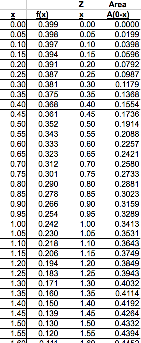
screen shot of spread sheet showing normal Z table

Spreadsheet 'Z-Table' resulting from coarse Trapezoid Slices
Figure 4 The material above has presented the results of a course computer model using the trapezoidal integration rule. While the model is simple, accuracy to three decimal places has been achieved. The student is encouraged to compare a few 'key locations' (such as z=1) between the model results in Figure 4 and the accepted results extracted from published statistical material shown in Figure 5 below. 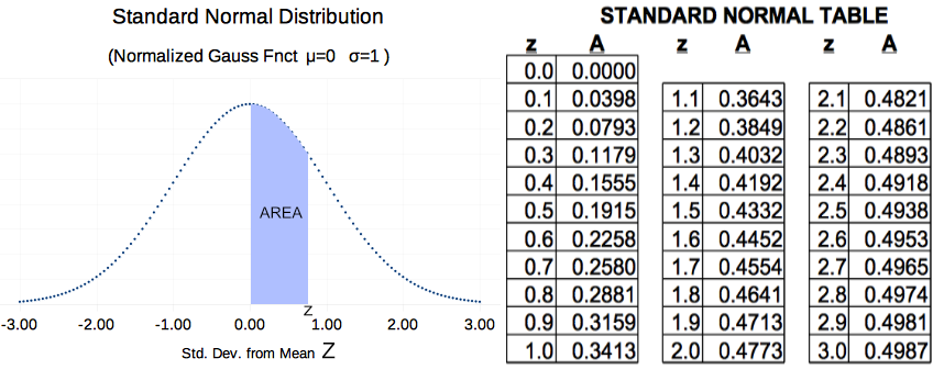screen shot of spread sheet showing normal Z table & illustration of Gauss PDF

screen shot of spread sheet showing normal Z table & illustration of Gauss PDF

Textbook Values of Z-Table
Figure 5 Figure 5 above is an actual Z-Table with Graphic PDF extracted from a statistics book. The student should note small errors made in the 'trapezoidal model' that resulted from the rather course number of slices.

Beginning of St. Pauls Statistics Introduction

Dionysus.biz Home Page