How Do We Compute xBar & s? What are they???

St. Paul's Statistics Introduction: Chapter 5

Calculating Mean and Standard Deviation from Data Sets

Section Goals:

• Students will learn and demonstrate methods to compute sample mean (xBar) and sample standard deviation s from datasets.
• Students will understand and be able to explain the difference between xBar and mean μ
• Students will develop conceptual understanding of how μ relates to a PDF

Introduction: In chapter 4, we worked many problems with the Gaussian Distribution and they always required us to know the mean μ (average) and standard deviation σ for the population of 'things' we were analysing. Chapter 4 identified three sources of those values:

1. Very well established theories, such as those in Physics.
2. Copious amounts of data (that's how the Physicists got their values)
3. Values calculated from data samples. When we use this approach, we refer to the sample mean (xBar) and the sample standard deviation (s). We do not use the symbols μ and σ when the values are computed from small to medium data sets.

Computing xΒar (imposter for μ): Please recall that μ is the average value for every item belonging to the population. If we are talking about the length of large construction nails, then μ is the average of length for every 16d size nail produced from Columbus up through the 22nd century. We would measure and add up all the lengths, and then divide the answer by the number of nails.

If we are talking about the weight of Cows, then μ is the average weight for every cow from the time of Moses up through the 22nd century. We would add up all the weights, then divide by the number of cows. We would need a time machine go back and weigh every cow because Moses lived a very long time ago. For most populations, it simply is not possible to get population data to compute μ. That is the reason we have to work with sample values xBar and σ.

So, how do you find the mean of x? Just add up all the x values, and then divide by their number. If you use 'all of them', then you get μ. If you use a sample of them, you will get xBar.

Brands & Prices for Peanut Butter
Chapter 5 Table 1

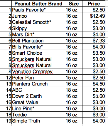
We can compute the sample mean 'xBar' based on the 19 prices in Table 1. Likely, you know the method, but here is the example:

Presenting Data - A Better Way: From Table 1, it is not obvious, but prices range from $1.50 to $12.99 for a jar of peanut butter. It is not obvious, but Table 1 has 6 products priced at $2.50.

• There are better ways of presenting the data so these observations are obvious.
• The data can be presented so we can more quickly find the sample mean.

Peanut Butter - Sorted by Price
Chapter 5 Table 2

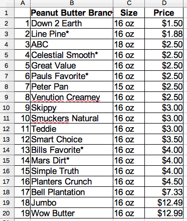
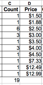
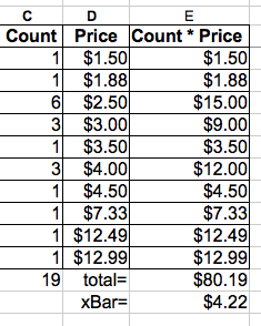
Further simplifications are possible. To compute xBar (the imposter for μ), we don't need the names of the peanut butter and we don't need jar size. Repeat entries are handled as shown in Table 3 below:

Price Data Sample Tabulated by Count
Chapter 5 Table 3

An Easier Way to Compute xBar: Based on Table 3, we can compute xBar either by calculator or by computer spreadsheet. We simply multiply 'Count' by 'Price' for each row in Table 3. Typically, these values are inserted into a new column to the right. Then, we 'total down' the new column. Finally, divide by the total by count of data items (19 in this example). Confused? We are just adding up all the Price numbers of Table 2 in a smarter way!

For a table with 19 data entries, it is not very important how you do it. But in the real world, statistics problems often have 150 data rows. For situations like this, it is impossible to look at the data table and draw any kind of conclusion. The data table must be sorted and repeat entries should be documented in a 'Count' column (like Table 3). This approach also makes computation of xBar much faster.

Reduced to math notation, this 'easier way' to compute sample mean looks like this:

Spreadsheet Form of Simplified Mean Computation
Chapter 5 Table 4

Homework Problems Chapter 5 :
For problems 1 through 4, use the data set to do the following. You may use either calculator or computer spreadsheet. Show all work.

• Read summary description of the problem.
• Sort the data into order (if it is not already)
• Group similar values (if any) and add 'count' column for repeated data values
• Do the math to compute sample mean xBar. Document all work & turn in to your instructor (if you have one)

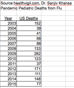
Chapter 5 Problem 1:
A Washington 'think tank' is encouraging larger budgets for health research. They want to statistically describe U.S. child deaths from Flu. Data from National Institute of Health follows

Child Deaths from Flu
Original Source: National Institute of Health
Chapter 5 Table 5

Concrete Strength Test Results
Chapter 5 Table 5

Banded Data: Very often, data is tabulated as huge lists of items with one entry per row. For example: Paul bought a pair of size 9 shoes → that appears as one data row. Tommy bought a pair of size 9 shoes → that is a different data row. When data items arrive as separate line items, but clearly many of the entries are similar, it makes sense to sort the data, and then group all the size 9 purchases together. It is very common to arrange data into 'bands' that fall into certain value ranges. For shoes, it seems very natural; but 'banded' data is quite common even when the 'x' variable seems continuous and repeats in the data are not evident. We will explore this topic when we study histograms in Chapter 6.

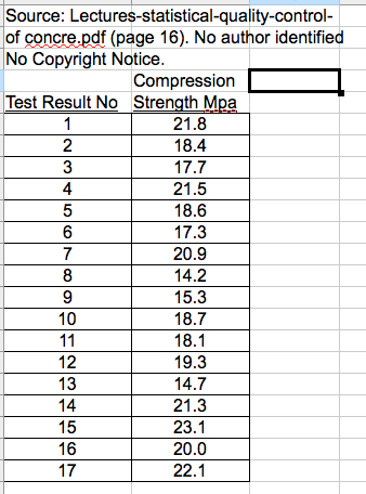
For problems 3 and 4, the data has already been sorted and grouped for you. Ignore the columns of data you don't need. Compute the mean of the data set.

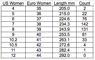
Chapter 5 Problem 3:
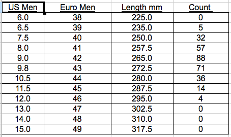
Shoe manufacturers are very interested in knowing the percentage of each shoe size sold so they can manufacture shoes in the proportions demanded by the market. Below, is a sorted data set that shows a sample of women's shoe purchases. Find the average.

Woman's Shoe Sales by SIZE
Chapter 5 Table 7

• Original Source: https://www.quora.com
• Data adjusted for equivalent US and European sizes.

Man's Shoe Sales by Size
Chapter 5 Table 8

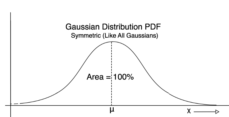
How is the Mean μ Related to the PDF? I offer a few PDF pictures with the mean shown on the graph. The mean of the PDF graph is always the balancing point! These four images illustrate that idea.

A Gaussian PDF Mean
Chapter 5 Figure 1


A Symmetric Triangular PDF Mean
Chapter 5 Figure 2


A NonSymmetric Triangular PDF
Chapter 5 Figure 3


NonSymetric PDF (Possibly Weibull)
Chapter 5 Figure 4

Mid Chapter Summary:

• We have learned how to calculate the sample mean xBar (which is often used in place of μ because we don't have a really good knowledge of the true μ value for the population).
• We have learned that we can look at a PDF, and make a good guess where the balance point is. And that location is also the mean.
• Those two ideas are pretty clear; but, there does seem to be a mystery. How do 19 peanut butter prices turn into a nice smooth curve likes Figures 1 through 4 above? We will explain the mystery of 'smoothing peanut butter' in the next chapter!

The Variance σ and imposter s:

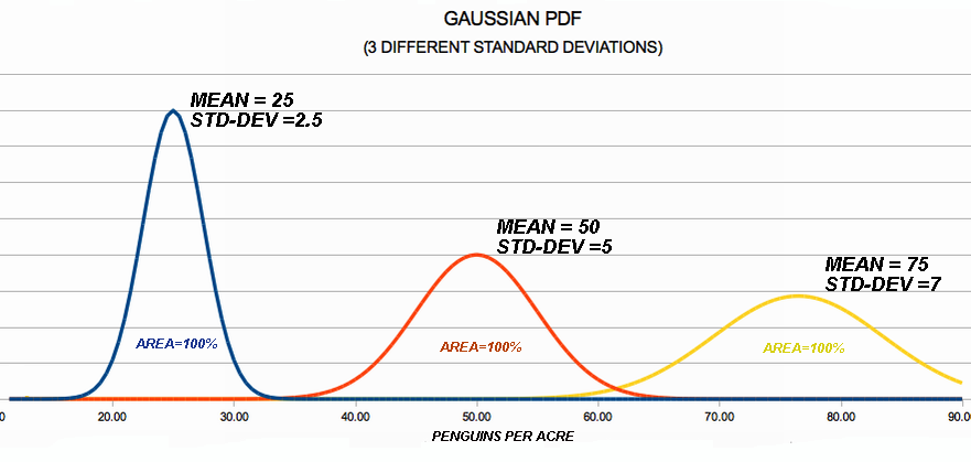
We know from Chapter 2 that the standard deviation σ determines 'how wide' the Gaussian PDF is. Chapter 2 Figure 3 is repeated below to refresh your memory. From the figure below, you should get the idea that:

Bigger Standard Deviation σ = Wider PDF Curve


3 Different GAUSS PDFs with Difference Variance
Ch 5 Figure 5

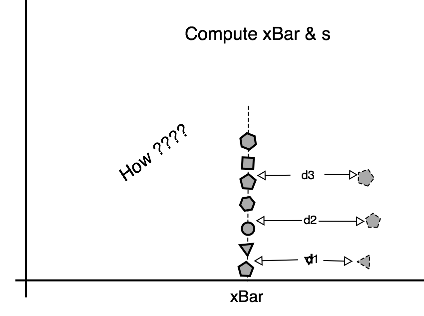
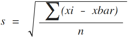
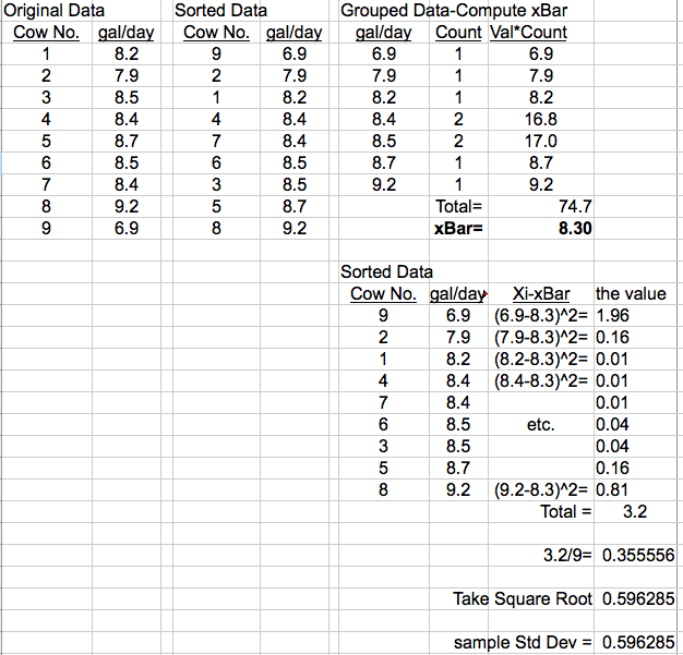
Computing s (imposter for standard deviation σ): In the real world, you usually won't know the standard deviation σ. You will have to compute an estimate based on a sample of data. A sample based variance is usually denoted 's' which is a way of reminding us that it is not the true, population value σ. s is an imposter that pretends to be the variance σ and we can use it in calculations in place of σ. In mathematical notation, the following equation defines how the sample variance s is computed:

1. Obtain a sample of data. It might be a list showing 9 cows. For each cow, a property of interest (like milk per day) will be documented. e.g. cow No 1 → 8.2 gal etc. for every cow
2. Compute the sample average value xBar using methods presented earlier in this chapter
3. For each data item (i.e. for each value xi) , we subtract xBar from it. And square the result.
4. Next, add up all the squared results
5. Divide by the number of data entries (n)
6. Take the square root

Calculating Sample Standard Deviation
Chapter 5, Figure 5

Homework Set 2 Problems Chapter 5:
Problems 5, 6, 7, & 8: Computation of Sample Standard Deviation s:

For each of the data sets of Problems 1,2,3 & 4, Compute the sample mean and sample standard deviation using the method shown above. You may use either calculator and paper, or spreadsheet.

Turn in the results to your instructor.

End of Chapter 5

Contact the author paul-watson@sbcglobal.net by e-mail.
© 2020 All Rights Reserved
Paul F. Watson

Beginning of St. Paul's Statistics Introduction
Dionysus.biz Home Page