St. Paul's Statistics Introduction: Chapter 2

Probability Density Function Shapes and Significance

Section Goals:

1. Familiarize students with the shape of several Probability Density Function (PDF) graphs.
2. Help students grasp the significance of PDF shape.
3. Make students aware of features common to all PDF graphs.

• The Two Dice Statistical Distribution
• The Binomial Statistical Distribution
• The Gaussian Statistical Distribution
• The Weibull Statistical Distribution

Please remember that a PDF is a pictorial representation of a statistical distribution and provides clues on how to get useful answers. A PDF is thus a kind of map. Actual answers are cranked out using math methods presented later (chapters 4,5 &6), but understanding the PDF will help you do the math and understand the answers.

Characteristics of a PDF:
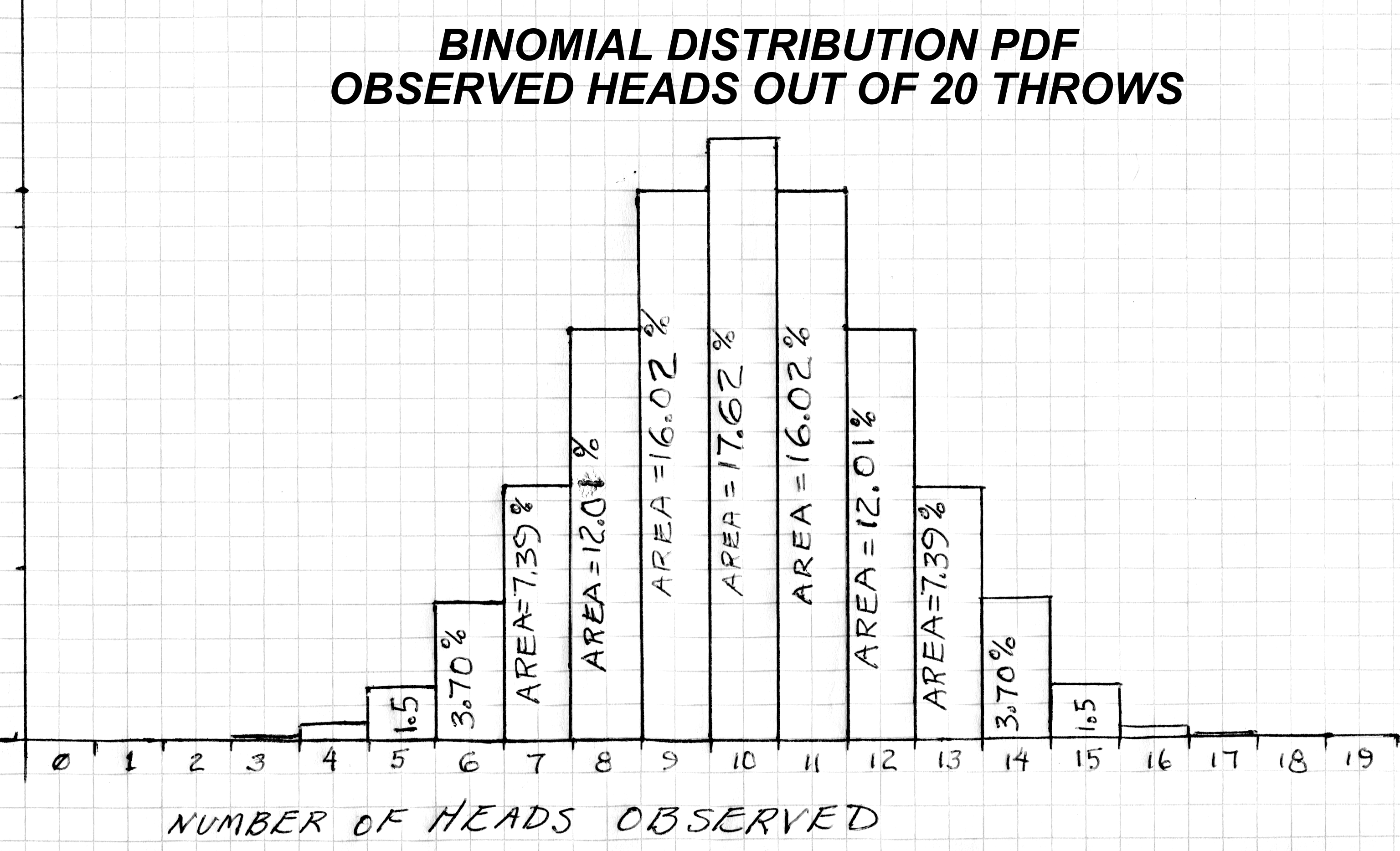
A Probability Density Function (or PDF) is a graph that describes the likelihood of different outcomes for a chance event. Consider flipping 20 coins. You would expect about 10 heads (and 10 tails). But you would not be surprised if the result were 12 heads on Tuesday or 9 on Friday. The PDF for coin flipping describes the likelihood of both these results AND it also shows a very small likelihood (almost zero) of getting 2 or 3 heads etc.. The PDF is presented below:

Ch 2 Figure 1
Probabilities of 'Heads' Out of 20 Coin Trials

The coin flipping PDF shows all possible outcomes (which of course totals 100%). For a PDF, the area under the curve represents probability (don't look at the Y value). From Ch 2 Figure 1, we can surmise that the probability of getting 9, 10 or 11 heads is 49.6% (add the three center bar areas). The probability of getting 0 or 1 heads is remote (almost zero percent).

PDFs for all distributions are interpreted in similar manner. Please note that on any given day, the observed results of a random event may be different; but, on most days, you will observe results where the large areas indicate high probability of occurence.

Homework: Ch 2 Problem 1:
Part a: Using the the PDF Ch2 Fig 1, what is the probability of getting 8, 9, 10 11 or 12 heads?
Part b: What about 10 or less heads?
Part c: If you throw 20 coins, what is the probability that 'something' will happen?
Part d: If you used only 1 coin, stuffed it in a box and shook it around before throwing it. And you repeated it 20 times, should you treat the total result as a single throw of 20 coins? Would that kind of process also obey the PDF Ch 2 Figure 1?

The Binomal Distribution PDF

• An aircraft flight control system is controlled by four computers, each performing the same calculation. Each computer checks its answers against those of its brothers. The probability of any computer failing during a flight is .01 percent (that is .0001 fraction). The aircraft can fly safely with only two operational computers. What is the probability of an aircraft having more than 2 failures during a flight?
• A WWII battleship could survive four torpedo hits without sinking. If 10 torpedos are fired, each with a 35% chance of hitting, how likely is it that the ship will be hit five or more times?
• Johnny's class has 15 students. School records show that about 10% of students fail the class. How likely is it that exactly four students will fail?
• A bolt factory produces batches of 12 specialty bolts. Over the last year, about 10% of bolts were rejected by Quality Control. Faced with four failures from a single batch, the plant manager wants to know, "Is this likely, or should I investigate what has gone wrong with the process?" OPTIONAL: Detective Statistics - The Negative Case
• During the Russo Japanese War (date: 1904), battleships fired groups of 4 cannon shells (called salvos). If the probability of one cannon shell hitting the target is 20%, what is the probability that two shells out of a salvo will hit? How about 3 shells? This method of firing, and mathematics of analysis were used in WWI and WWII as well.

OPTIONAL: Forensic Statistics Use - The Negative Case. Detectives look for something 'out of place' at a crime scene. Can statistics be used in the same way?

Criteria for Using the Binomial Distribution
When the following four conditions are ALL true, the Binomial Distribution can be confidently used.

• The number of trials is known and (usually) less than 12 (e.g. 4 computers, 10 torpedoes, 12 bolts etc.) Note: There is nothing wrong with using the binomial for 20 or 30 samples, but you will be calculating all day long. For problems with more than 12 samples, computers are used, but even with computers, binomial analysis can result in very, very large numbers that may "choke" the computer. In 1978, the Apple computer could handle numbers as large as 1 followed by 36 zeros. in 2019, the Python computer language can handle numbers as large as 1 followed by 300 zeros. Don't be surprised if you exceed even Python's abilities when working with large binomials.
• Each trial has a binary result (i.e. a torpedo hits, or does not hit. A student fails or does not fail, A student eats liver, or does not)
• The probability of 'success' is known (e.g. .15%, 35%, 50% etc.)
• The success of each trial is independent of the other trials. This means that after a torpedo hit, the next torpedo is neither more, nor less likely to hit.)

Homework: Ch 2 Problem 2: Using the four criteria above:

1. Decide whether or not the binomial distribution can be used to analyze the toss of 10 coins that was discussed above (yes or no). Look at Ch 1 Fig 1 which statistically describes this situation.
2. Write a brief list of steps that justifies your answer.

Compare your analysis to St. Paul's. Click here for Paul's solution.

Homework: Ch 2 Problem 3: Using the four criteria above:

• Decide whether or not the binomial distribution can be used to analyze risk to a small dairy farmer. He has 10 cows. Each cow has a 2% chance of producing bad milk. To pay his mortgage, all 10 cows must be good producers. The farmer wants to know the likelihood that all 10 cows will be good? How likely is it he will have 1 bad cow?
• Write a brief list of steps that justify your answer.
• e-mail your conclusion and reasoning to your instructor.

How Many PDFs does the Binomial Have?
The following paragraph will begin to familiarize the student with the trends of the binomial distribution. Please read the material, try to make sense of it and move on. Don't waste time memorizing the details of this figure. Just try to understand the general idea.

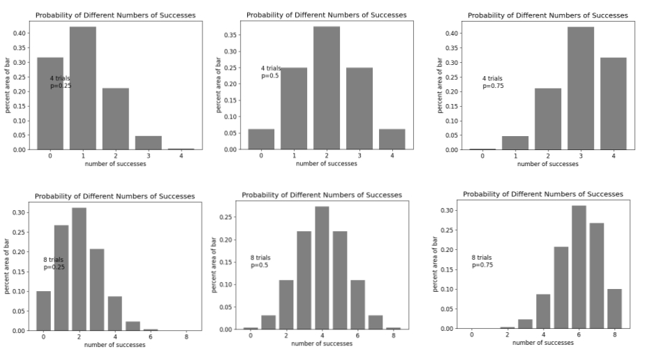
The Binomial is actually a family of PDFs. All 8 PDFs below (see Ch2 Figure 2) are members of the Binomial Statistical Distribution. A binomial is mathematically generated, based on the probability p, and the number of samples n. Thus, each different value of the n,p number pair will generate a different PDF; but, all the PDFs do look rather similar as shown below:

Binomial PDFs - Variation of Parameters n,p
Ch 2 Figure 2

1. For the binomial family of PDFs, the general shape is similar. The PDF in all cases is much like the cross section of a bell; but, it is sometimes distorted.
2. The binomial above is discrete -- i.e. the x axis represents only counting numbers (0,1,2,3 ...) and no fractions.
3. When n is larger, the PDF remains the same general shape but has more bars and becomes smoother.
4. The value of p, determines the distortion of the "bell" shape. p determines if the PDF is skewed left, right or is symmetric.
• If p less than 50%, then PDF is skewed right meaning that success end of the graph is "starved". For the top left graph, since average probability is only 20%, we should not expect a lot of successes.
• If p equals 50%, then PDF is symmetric meaning multiple failure and multiple successes are equally likely.
• If p greater than 50%, then PDF is skewed left meaning the successes are concentrated at the "many" end of the probabilities.
• There is actually a skew number that describes how "lopsided" the histogram is - but we won't go into that.

The Gaussian Distribution PDF

Very often, the Gaussian is simply "presumed" to be appropriate and is applied to data. Then, engineers and scientists do a reasonableness check before proceeding further. Below are three examples of phonomina where the Gaussian distribution applies and two examples where it does not work well.

• The IQ test was invented during WWI to help place solders into appropriate jobs. The IQ scores of a large sample of people is known to follow a Gaussian distribution.
• When production lines manufacture parts (bolts, brackets, pistons, bearing rings etc.) it is routinely assumed that every dimension on the manufactured part will statistically vary according to a Gaussian distribution. This assumption has proven useful over time and is basis for statistical process control.
• A botanist's first guess would be that leaves off a certain oak tree would vary in a Gaussian fashion.
• Counter Example: For many products (such as computers), it has been noticed that failures of "new" items are common. But if the item survives the first few months, it is good for years. This kind of failure is called "infant mortality" and is usually modeled with Exponential Probability Distribution. (The Gaussian can not handle this)
• Counter Example: The wear-out life of a "jack hammer" piston is likely not Gaussian. Wear-out is the result of friction and metal fatigue. These kinds of phenomena are typically fitted to a Weibull Distribution. (Gaussian cannot handle this one).

We just looked at some populations which are Gaussian and some that are not. Below are two clearly stated examples of industrial problems that can be solved using the Gaussian Distribution and methods that will be presented in Chapter 4. Chapter 4 will also explain the technical terms mean μ and "standard deviation" (sigma). Chapter 4 will show you how to compute the mean μ and standard deviation (sigma) for a sample of parts coming off a production line.

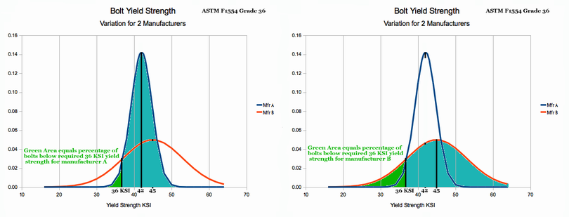
• Percentage of Bad Product: A bolt factory makes foundation bolts that are supposed to comply with industry standard ASTM F1554 Grade 36 which requires a minimum strength of 36 thousand pounds per square inch (36 KSI). Trial runs from the production line show a mean μ (or average) bolt strength of 45 KSI with a standard deviation σ of 8 KSI. If adjustments are not made, what percentage of bolts produced will fall below the required strength? (Gaussian can do this)
• An armaments manufacturer makes cannon shells. The amount of propellant must be controlled carefully so that all shells are accurate. For a small howitzer shell, the production line can provide 8.1 pounds of propellent (the mean μ) with a standard deviation (σ) of .2 pounds. The specification requirement is that propellent must be between 8.0 and 8.2 pounds. What percentage of production shells will fail to meet the requirement? (Gaussian can do this also)

How Many PDFs does the Gaussian Have?
The following paragraph will begin to familiarize the student with the behavior of the Gaussian distribution. Please read the material, try to make sense of it. The student should read and re-read the material until the general trends of mean and standard deviation are committed to memory. You want to concentrate on understanding the trends. Do study the fact that increases in mean (μ) from 25 to 50 to 75 slide the "bell shaped curve" to the right. Do study the fact that in the second row, increasing the Standard Deviation from 2.5 to 5 to 7 stretches the curve in the horozontal.

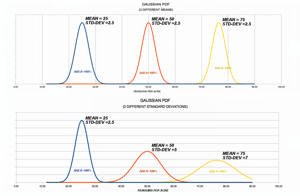
The Gaussian Distribution is actually a family of PDFs. All six of the curves (Fig 3 below) are Gaussian. A particular Gaussian PDF is mathematically generated, based on the average value (mean μ), and the standard deviation σ (which will be mathematically explain in Chapter 4). Thus, each unique pair of parameters (mean σ, StdDev μ) can be used to generate a corresponding Gaussian PDF; and yet, all the PDFs do look rather similar as shown below and handled by the same math:

Ch 2 Figure 3
Effect of Changing Mean & Standard Deviation of a Gauss PDF

The Gaussian Distribution has a family of PDF curves, each being defined by its mean and standard deviation. The figure above (Ch 2 Figure 3) provides the student with a clear illustration of how the PDF changes as the mean increases. Basically, the Gauss PDF shifts off to the right so its center aligns with larger and larger values of the mean. If the mean value is increased, the entire PDF slides to the right and all the bolts have higher strengths. This concept proves very useful because on Tuesday our bolt factory may be making 36 KSI strength foundation bolts; but, on Friday we may be making high strength 150 KSI aircraft bolts. We can use the Gauss PDF model for both by simply adjusting the value of the mean!

The Gaussian Distribution has a second parameter- the "so called" standard deviation (σ) which we will study in Chapter 4. Looking at the lower part of Ch 2 Figure 3, we can see the effect of varying the Standard Deviation. The lower left graph has a standard deviation of 2.5, and is narrow. The total area under the curve is still 100%, but all the area is fairly close to the central mean (μ) value. In practice, this means that when such bolts are sent to build foundations, the strength values of all will be pretty close to the mean value (because all the PDF area is close to the mean value).

Examining the lower middle graph, the area is still 100%, but the graph is wider and shorter because the Standard Deviation has increased. This means that bolts built with this kind of Gaussian PDF, will put bolts with considerable strength variation into buildings and airplanes they are intended for (not so good). The lower right graph is wider still indicating large variation in properties of the bolt or other product it describes. In general, industrial processes with a large standard deviation are not a good thing.

We will study the significance of varying mean and/or standard deviation in Chapter 4; but, for now, the student is to understand that the Gaussian PDF has the ability to describe items with high values of strength, ductility, or penguin population. The Gaussian PDF is also capable of describing situations where there is little to much variation in the observed quality be it strength or Penguin population.

OPTIONAL: Some might wonder "Why can't I just make it the way I want and to heck with the mean and standard deviation!

Observations about the Gaussian PDF

• The X axis is a full number line with decimal fractions (It certainly has numbers like 1, 2, 3 ... but it also has everything in-between. Unlike the Binomial, it has numbers like 2.8, 5.325 and all that).
• Unlike the Binomial, it is not a discrete distribution. As a result, the area under the curve is probability. The value on the Y axis has little meaning.
• For your information, the Gaussian PDF is officially defined by an equation. The very nice illustrations were created on a spreadsheet by using Gaussian equation.
• Chapter 4 will explain the math of the Gaussian, and how to use it to solve industrial and historical problems.

The Weibull Distribution PDF

• The severity of Japanese earthquakes (I have not examined US earthquakes)
• The height of tidal waves recorded during the last 400 years.
• The size of particles in a smoke stack
• Yield strength of Bofors steel
• Fiber strength of Indian cotton
• Typically, the life of brearings, brake assemblies and mechanisms.
• The fatigue life of solder joints inside your computer
• and many others

The Weibull Distribution was discovered in 1927 by Frecht but was not widely known until 1951 when Swedish Engineer Walodi Weibull wrote a short paper explaining its usefulness. Like the Binomial and the Gaussian distributions, the Weibull distribution has well established methods of use. It is a bit more difficult to use than either the Binomial or the Gaussian distributions; but, is extremely powerful because of the wide range of problems it can solve.

Like the Gaussian Distribution, the Weibull PDF is generated by an equation. The x axis is continuous and as a result, areas under the PDF are equivalent to probability. The Y axis PDF values have little or no meaning.

How Many PDFs does the Weibull Distribution Have?

1. Two parameter Weibull that has slope parameter Beta β and (Characteristic Life) parameter eta η
2. Three parameter Weibull that has slope parameter Beta β, characteristic life parameter eta η and initial event time tzero

What Does the two parameter Weibull PDF Look Like? Ch2 Fig 4 below presents 4 Weibull PDF graphs, with different Beta β values (.5, 1, 1.5 and 2). In some way, we can say that these curves look similar, but as Beta β changes, the Weibull PDF takes on different shapes. All 4 curves are drawn with eta (η)=35. Increasing the eta (η) value stretches the curve horozontally.

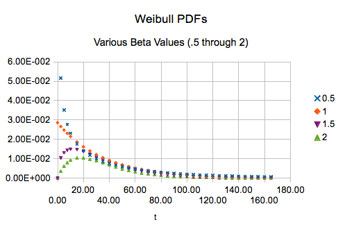
Ch 2 Fig 4

Definition of the Weibull PDF: The Weibull Probability Distribution is defined by the following PDF equation:

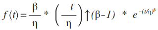
Ch 2 Fig 5

Chapter 2 Summary: In chapter 2, we discussed three industrially useful Probability Density Functions.

1. Binomial
2. Gaussian (or Normal)
3. Weibull

• Log-Normal
• Student t
• Poisson (Very nice. See Note Below:)

End of Chapter 2

Please use the BACK ARROW at top left of your browser to get back to the main statistics lessons.