The definitions page will be made available throughout this course. The words are in alphabetic order, so please scan down the page to find the word you are looking for.
Event = something that happens. In statistics, events are happenings where the result can be measured or counted. Statistics deals with numbers, not value judgements.
Gaussian Probability Distribution: First, what is a probability distribution? A probability distribution is a blue print or pattern of how probabilities are matched to outcomes of some event. Let's clarify that idea of a probability distribution before we explain a particular type, the Gaussian Probability Distribution.
The example that follows is not Gaussian, but its shape is very similar. Consider the probability distribution, that would describe 50 coins thrown in the air, and the number of heads are counted after they land. The distribution would tell you the percent of throws that produces 25 heads. It would tell you the percent of throws with 26 heads. It would tell you the percentage of throws that would result in 27 heads. In fact, the distribution would match a probability to every possible throw count (0 through 50). This is usually done by either a PDF graph, or by an equation (note that an equation can be used to draw a graph.)
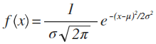
Next, let's define the Gaussian Probability Distribution. It is the very common, "bell shaped" PDF curve. The Gaussian PDF is actually defined by the equation shown below:
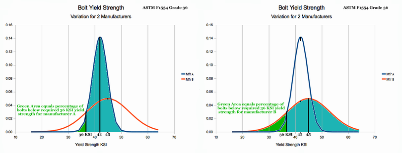
PDF graph (or probability density function graph) is a picture representing all of the possible state outcomes that can result from some event. The possible outcomes are listed across the x axis, and the area above the x axis indicates the probability of occurrence. Unlike the usual math graph, AREA is important --- not y value. It is difficult to comprehend from words, but examples provided in Chapter 2 will clarify this concept.
Population = the entire family of similar objects that have ever been made, or will ever be made. If we are talking about 1/4 inch bolts, then the population is made of either:
Probability = the likelihood of a specific outcome from an event. The probability is usually expressed as a percentage (e.g. 25% likely). The percentage indicates the result which is expected after a very, very large number of events.
For example, a coin toss is 50% likely to end up heads. This means that if we throw a million coins, we should expect pretty close to 50% of a million or 500,000 heads. If we throw 100 coins, we should expect 50% of 100, or about 50 heads. As the number of coins thrown gets smaller, the predicted number becomes less accurate.
State = refers to the overall situation with regards to a group of objects. State implies little or no concern for individual identity of the objects; but refers only to the impersonal description of how many are in what condition.
Example 1: Consider 5 coins, named Albert, Beth, Charlie, Dianna and Ed. One possible state is 2 heads and 3 tails. When we talk about state, we are not concerned with the names of the 2 that are heads. Our level of concern stops with the impersonal observance of 2 heads and 3 tails.
Statistics tends to be confusing. One of the reasons is: As we approach a problem, we may have to think in very small detail about what can happen (e.g. how many combinations of Albert, Beth, Charlie, Dianna and Ed are there that result in 2 heads?). It is hard to know unless you write them down - by name. But the final answer rarely is concerned with that level of detail. Thus in the early stages of a problem, we must often think in small detail, but the final answer requires thinking at a much more general level. This switching back and forth combined with the large number of "specialty words" used in Statistics makes for a lot of confusion. In this course, we will try to be as clear as possible and will use as few "specialty terms" as possible.
Example 2: If we consider 10,000 molecules in a cubic inch of air, the state might be the number of molecules that travel at different speeds (10-20 mph, 21-30 mph ... 91-100 mph). All 10,000 molecules may have names and personalities; sorry to offend, but we really do not care. Description of the state stops with the impersonal description of how many are in each speed bracket.
It is a bit like the political process. Every voter has a name and personality; but, the election result is a raw count of votes for each candidate (and ignores who voted Republican vs. who voted Democratic ...)
A Statistical Distribution: is a "blue print" or pattern that relates states to probability of occurrence. The pattern can be defined by a graph like the ones I am showing you in the course. The pattern for some Statistical Distributions can also be defined by an equation.
The equation form is often used because Calculus Mathematics is very good at computing area underneath a curve which is defined by equation. This is primarily true for Statistical Functions where the x axis is a continuous number line which includes decimal fractions (e.g. 1, 1.1, 1.15, 1.3, 1.567, 2, 2.1, 2.34 ... and everything in between.
So we might conclude by saying that if we have 5 equations, each representing a statistical distribution, then we have five different blueprints and hence five different statistical distributions. When they are graphed, they usually look different from one another. By simply looking at a PDF, it is often obvious what distribution it is.
Success vs. Failure: An event often results in "success" or "failure". If a boy gave a ride to his girl friend and ran out of gas, he might call that success because he would enjoy the long walk back to town with his friend. The girl might call it failure because she secretly had a date with someone else, and needed time to get ready.
So the result tagged as success is a matter of viewpoint. During statistical analysis, it does not really matter which result you call success (running out of gas, or not), but once you start the problem you mustn't change your definition. Stick to it until the final answer is computed. If you follow that approach, you will get the right answer.
Usually, the probability of success is represented by variable p, and failure by variable q. That is simply the way most teachers and writers do things. We will stick to this convention as it will make understanding the work of others a lot easier if we use the same terminology.
Trial:When we talk about statistical distributions, we are talking about the percentage occurrence of each outcome were we to repeat an event (or an experiment) many, many times.
Each time we do an event (or experiment), we only get one result. So it is necessary to repeat the experiment thousands of times to build up a record that matches event to percentage occurrence. Each time we repeat the event of interest, that is called a trial.
For the dice problem in Chapter 1, it was not necessary to do thousands of trials in order to create a Probability Density Function. Why? The probabilities of different dice roles are simple and well understood. It is possible to use math and compute the probability of various outcomes without performing any experiments. Some problems are like that, but other problems require hundreds if not thousands of trials to develop a good estimate of the PDF.
Conclusion: A trial is a single experiment that meets some description of an event (event being the idea or happening you are exploring.) Often, hundreds of repetitions of an experiment are needed to make good statistical conclusions. In the language of statistics, hundreds or thousands of trials may be needed to characterise the probability density function (PDF) of an event.
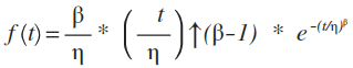
Weibull Probability Distribution Function: the Weibull Probability Distribution Function is defined by the following PDF equation:
Contact the author
paul-watson@sbcglobal.net
by e-mail.
© 2019 updated 2020
All Rights Reserved
Paul F. Watson