Statistics and the Probability Foundation: Chapter 1

The Birth of Statistics (Probabilities Stacked on Probabilities)

Section Goals:

1. Define two fundamental laws of statistics & one Corollary.
2. Utilize two fundamental laws to compute likelihood of various dice roles on two dice.
3. Construct a Probability Density Function chart using computations from above.

The Birth of Statistics:
Probability math was begun when French gamblers approached a great French mathmetician a few hundred years ago. Gradually, Statistics grew out of Probability Theory to where we are today. Our first example will start, as Descartes did, with dice. We need that background; but, Chapter 2 will dive into Industrially Useful statistics which are based on concepts presented in this chapter.

Ch1 Example 1: The Throw of Two Dice
Two dice (named "A" and "B") are thrown from a gambler's hand. Let's determine the probability that the total number of spots on the dice is two. This implies that Die "A" shows one spot. And Die "B" also shows one spot. There is no other way that a 2 can result from a pair of dice.

During the solution of these problems, two general laws will be used. The laws are stated below and their truth will become obvious as you work through Ch1 Example 1.

General Law 1: If the probability of one event is r (maybe 16%), and the probability of a different event is s (it could be 25%) then: Probability of Both Events Occuring = r x s. (e.g. for r=16% & s=25% then r*s=.16*.25 which is .04 or 4%)

General Law 2: If the probability of one event is r, and the probability of a different event is s, then: The probability that somebody (either r or s) = r + s (e.g. for r=16% and s=25% then r+s=.16+.25=.41 or 41%. Thus the probability of either r happening or s happening or both happening is 41%)

General Law 2 Corollary: When an event (or state) can occur in several different ways, the probability of the event (or state) is the sum of the probabilities for all the ways it can happen. This is a direct consequence of General Law 2 above since for three events, the first two can be taken first by summing the probabilities and then the last is added to the result. This argument can be extended to any number of such events.

The truth of General Laws 1 & 2 will become evident as we work through the 2 dice problem.

Solution:

1. For "A", the likelihood of throwing a 1 is 1 side out of 6 possibilities (1 divided by 6 = 16.67%)
2. For "B", the same reasoning indicates 16.67%
3. When "A" and "B" are thrown from the same hand (simultaneously)
• A & B are thrown together, but imagine a cardboard box covering the result. We slowly move the box to reveal only one die. Only 1/6 of the time will a 1 be revealed.
• So 1/6 of the time, we proceed to uncover the other die. For the 2nd die, we will only get the desired result 1/6 of the time.
• Thus, we will get the "one" and "one" result 1/6 of 1/6 of the time: 1/6 x 1/6 = 1/36 or 2.78% (alternatively, 16.67% x 16.67% = 2.78% which is the same answer)

The reader will observe this answer is in agreement with General Law 1 (plug in the numbers and punch it out on your calculator.) If you could find honest 8 sided dice, the logic of solution would be the same and the answer would once again be in agreement with General Law 1. The same is true for any number of sides, and we shall now consider General Law 1 to have been proven.

Let's get some more practice with "stacked probabilites" before moving into the next chapter. So let's finish solving the two dice problem for all possible outcomes The possible outcomes for the throw of two dice are:

Now, determine the Probability of throwing a 12 with two dice (i.e. Solve Row 12):
Let the two dice be called "A" and "B". The only way to throw a 12 is for "A" to be 6 AND "B" is also 6. There is only one face out of six with the needed number of spots. So this problem is not mathematically different from the "1" and "1" example already worked. The answer is 1/6 x 1/6 = 1/36 or 2.78% just like we got before! YOU there. Go fill in the last row of the table with 2.78% !

Next, determine Probability of throwing a 3 with two dice (i.e. Solve Row 3):
We can get a 3 dice role in either of two ways. Either a 1 and a 2 for A & B, or vice versa.

Now, we apply General Law 2. A 3 is achieved by EITHER of the rows. Hence the probability of " this or that" is 1/36 + 1/36 which is 2/36. On the calculator: 2 divided by 36 = 5.56%.

YOU there. Go fill in another row of the table you are copying into your notebook. We are going to need that table in a little while.

Now, determine the probability of throwing 11 with two dice:
Careful consideration shows this solution is exactly like the one above. We can get an 11 with either five and a six, or vice versa. The math and everything is just like "row 3" and the probability is 5.56%. So go fill in "Row 11" in the table you are making.

Now, determine the probability of throwing 4 with two dice:
There are three ways to get a 4 with 2 dice. They follow, along with the calculation of probability for each of the rows. For the final probability, it is the sum of the probabilities in the right hand column (because we don't care how we get a 4. We just want a 4 regardless).

We now now the probability for each way we can get a four. In accordance with General Law 2, we add the probability for each way (i.e. 1/36 + 1/36 + 1/36 = 3/36) which equals 3/36 or 8.33%. YOU there. Go add that into the table you are making.

CH 1 Homework 1:
Go work out the probabilities for each of the following. Add them to the table we are building"

• Find the probability of rolling a 5 with two dice. Hint: list all the ways it can be done first. Add the result into the table you are building.
• Find the probability of rolling a 6 with two dice. Hint: list all the ways it can be done first. Add the result into the table you are building.
• Find the probability of rolling a 7 with two dice. Hint: list all the ways it can be done first. Add the result into the table you are building.

The bottom of your table will be mirror images of the top. The finished table will look like Ch 2 Table 4 shown below. Check your answers. If you got them wrong, try again.

We just gained insight into how the number of ways an event can occur influences outcome probabilities. We also used General Laws 1 and 2 to compute probabilities for dice roles. While these are useful, statisticians have developed graphic pictures that help us visualize "the big picture". These are called Probability Density Functions (or PDF for short). These pictorial diagrams will prove very useful -- particularly so when we get to the very powerful Gaussian Probability Distribution. (I should clarify that a Probability Density Function can be in either graphic form, or can be written as an equation. We will be concentrating on the graphical form).

Probability Density Function for Throw of 2 Dice
Ch 1 Figure 1

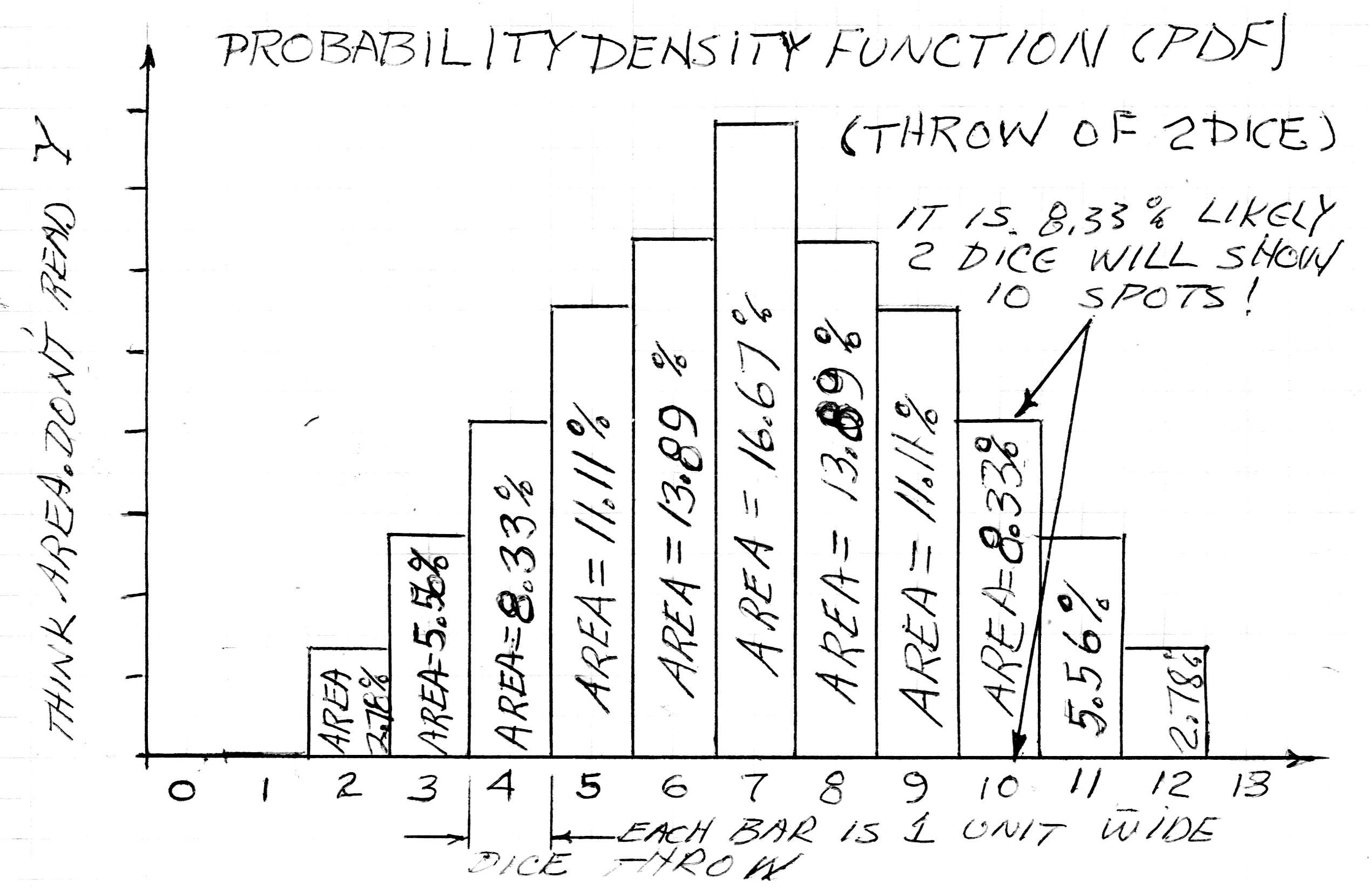
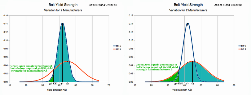
Observations about the PDF for 2 dice:

1. Every possible outcome of the dice (2 through 12) is represented.
2. For the dice example, numbers on X axis are counting numbers (1, 2, 3 NOT 2.8)
3. Each bar has a width of one. (i.e. The bar labeled 4 is the 4th bar. But these are counting numbers. The 4th bar represents exactly one more than the previous bar. We count outcomes like we count bananas (i.e. 1, 2, 3). The 3 represents "the whole banana" (does not represent everything from 2.5 to 3.499999). The width of each bar is one unit!
4. Since the width of a bar is one, then the area of a bar is exactly the same as the height. In the future, when we use PDF charts for continuous number lines, we MUST think about Area --- not the Y value! This area concept will prove very useful in future lessons. For now, the PDF we are examining is counting numbers so the Y value and are Area are EXACTLY THE SAME!
5. The sum of probabilities for all the outcomes is 100%. Add them up for yourself! You may get 99.98% because of "round off error" in your calculator, but that is very close to 100%

In Chapter 2, we will examine PDF fuctions for several Industrially useful Probability Distributions. We will talk about the kinds of problems where those distributions are useful. Finally, we will also discuss what we can learn from the shape of the PDF.